← Systemic change, effective altruism and philanthropy

Hamiltonian systems and closed orbits in replicator dynamics of cancer →

Multiple realizability of replicator dynamics

June 9, 2016 by Artem Kaznatcheev 4 Comments

Abstraction is my favorite part of mathematics. I find a certain beauty in seeing structures without their implementations, or structures that are preserved across various implementations. And although it seems possible to reason through analogy without (explicit) abstraction, I would not enjoy being restricted in such a way. In biology and medicine, however, I often find that one can get caught up in the concrete and particular. This makes it harder to remember that certain macro-dynamical properties can be abstracted and made independent of particular micro-dynamical implementations. In this post, I want to focus on a particular pet-peeve of mine: accounts of the replicator equation.

I will start with a brief philosophical detour through multiple realizability, and discuss the popular analogy of temperature. Then I will move on to the phenomenological definition of the replicator equation, and a few realizations. A particular target will be the statement I’ve been hearing too often recently: replicator dynamics are only true for a very large but fixed-size well-mixed population.

Multiple realizability for minds and temperature

Multiple realizability is usually associated with the philosophy of mind. In this context, it is the thesis that the same mental property can be implemented by different physical states. That similar minds can be implemented by very different brains.^[1] But minds are not the only thing for which we should worry about multiple realizability. It is a concept that applies across the philosophy of science.

One of the most convincing examples of multiple realizability comes from physics: implementations of temperature. You might have learnt that temperature is mean molecular kinetic energy. This is true of an ideal gas, but the temperature in a solid is mean maximal molecular kinetic energy. In a plasma, temperature is yet another thing. These difference in implementation arise because the important features of temperature are macrodynamical and defined by analogy to substances where we already understand and care about temperature. In particular, a substance that is not an ideal gas is said to be at temperature T if it would be at thermal equilibrium with an ideal gas heat bath at temperature T. This means that the microdynamical details of temperature can be different for every new substance. Thermodynamics and other theories built on top of temperature are thus abstracted away from the microdynamical details of statistical mechanics.

I believe that replicator dynamics are multiply realizable in much the same way as thermodynamics. Where statistical mechanical details of thermodynamics differed in their implementation of temperature, microdynamical implementations of the replicator equation will often differ in their definition of fitness. There are a few theoretical systems like large constant sized populations or exponentially growing ones — the replicator dynamics equivalents of the ideal gas or square-lattice Ising model — where we can derive the replicator equation explicitly. In other models, we can use replicator dynamics empirically and by analogy, without having to worry about the details of a microdynamical implementation.

Replicator dynamics

On the macroscopic level, the replicator equation was introduced by Taylor & Jonker (1978)^[2]. This was based on the operationalization of fitness^[3] by the per-capita growth rate $\frac{\dot{x_k}}{x_k}$ of a strategy k as proportional to its relative fitness $w_k - \langle w \rangle$ (where $\langle w \rangle = x_1 w_1 + ... + x_m w_m$ is the average fitness of the population). Giving us the familiar system of equations:

$\dot{x}_k = x_k(w_k - \langle w \rangle)$

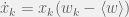
which is known as the Taylor form. Under a slightly different set of phenomenological assumptions, we can also get the Maynard Smith form (Maynard Smith, 1982):

$\dot{x}_k = x_k\frac{w_k - \langle w \rangle}{\langle w \rangle}$

where the extract condition of $\langle w \rangle > 0$ is introduced. In the limit of weak-selection, these two forms are equivalent. Even without weak-selection, the two systems of equations differ only by time distortion and thus have the same fixed points, orbits, and paths. Since these are often the things we care most about during typical analyses, we can use the equations interchangeably.

The realization of these equations can be left unspecified to remind us that many micro-dynamical reductions are consistent with this system of equations. Unfortunately, some realization are discussed more often, eclipsing other possible interpretations. I want to discuss three specific realizations in the remaining sections: well-mixed Moran processes on large constant sized populations, empirical growth rates of arbitrary experimental populations, and exponentially growing populations.

Fitness as probability to reproduce in populations of constant size

Replicator dynamics are continuous — in both time and probability — and deterministic. In lots of settings, however, theorists do not want to assume continuous dynamics, and instead use stochastic models like branching processes. This choice is justifiable because discrete stochastic processes and their continuous approximations are known to be qualitatively different in some settings; for a drastic example, see Shnerb et al. (2000). This discretization urge is further strengthened by the accessibility and prevalence of computational agent-based models, and the fact that many of the top theorists have a physics background and associated propensity to focus on insilications build up from a simple, well-characterized ontology.

The focus on individual agents pushes the theorist to look for definitions of fitness on the individual — rather than population — level. They find such a definition in the Moran process, and with it comes the realization of replicator dynamics as a process on well-mixed and large but fixed sized populations.

In a Moran process, we imagine that a population is made up of a fixed number N of individuals. Each of these individuals has some intrinsic payoff value. In the case of game theory, this payoff usually depends on the strategy of that agent and others in the population. An agent is selected to reproduce in proportion to that payoff, and their offspring replaces another agent in the population, chosen uniformly at random. This gives us a very clear individual account of fitness as a measure of the probability to place a replicate into the population.

Traulsen, Claussen, and Hauert (2006) write down the Fokker-Planck equation for the above Moran process,^[4] and then use Ito-calculus to derive a Langevin equation for the evolution of the proportions of each strategy $x_k$ . The fluctuations in this stochastic equation scale with $1/\sqrt{N}$ and so vanish in the limit of large N. This reduces them to a deterministic limit of the replicator equation in Maynard Smith form,^[5] with the fitness functions as the payoff functions.

The difficulty arises if you want to operationalize this model. Then you have to figure out how these fitness/payoff functions correspond to experimental measurements. How will you measure them at the individual and not population level? Here all that is gained from discretization can be lost in the blurriness of measurements.

Fitness as experimental growth rate

Instead, let us start at measurement. In particular, measurements of growth rates. In the case of cell biology, this is most often populations growing in Petri dishes. Unlike the previous section, there will be no constraitns on population size, but also no agent-based microdynamical story. Instead, we will receover replicator dynamics from purely in experimental outputs or their limits.

If you are running an experiment with some tagged cells of m many types: 1, … , m then your most basic primitives are (estimates of) the sizes of your seeding populations $N^I_1, ... , N^I_m$ and the size of final populations $N^F_1, ... , N^F_m$ . Given these values and a time difference $\Delta t$ between the experiment was started and when it ended, the microbiologist would define the experimental population growth rates as:

$w_k := \frac{N^F_k - N^I_k}{N^I_k \Delta t}$

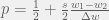
this can be rotated to give us a mapping $N_I \mapsto N_F$ :

$N^F_k = N^I_k (1 + w_k\Delta t)$

From defining the initial and final population sizes $N^{\{I,F\}} = \sum_{k=1}^m N^{\{I,F\}}_k$ , we can compare the initial and final proportions of each cell type:

$\begin{aligned} x^I_k & = \frac{N^I_k}{N^I} \\ x^F_k & = \frac{N^F_k}{N^F} \\ & = x^I_k \frac{1 + w_k\Delta t}{1 + \langle w \rangle \Delta t} \end{aligned}$

where $\langle w \rangle = \sum_{k = 1}^m x^I_k w_k$ .

So far we were looking at a discrete process. But often, it is convenient to approximate it with a continuous one for ease of analysis. In that case, we can define $x_k(t) = x^I_k,\;\; x_k(t + \Delta t) = x^F_k$ and look at the limit as $\Delta t$ gets very small:^[7]

$\begin{aligned} \dot{x} & = \lim_{\Delta t \rightarrow 0} \frac{x_k(t + \Delta t) - x_k(t)}{\Delta t} \\ & = \lim_{\Delta t \rightarrow 0} \frac{x^I_k}{\Delta t} ( \frac{1 + w_k\Delta t}{1 + \langle w \rangle \Delta t} - 1) \\ & = \lim_{\Delta t \rightarrow 0} x_k \frac{w_k - \langle w \rangle}{1 + \langle w \rangle \Delta t} \\ & = x_k(w_k - \langle w \rangle) \end{aligned}$

and we have recovered replicator dynamics and gave an explicit experimental interpretation for all of our theoretical terms.

Exponentially growing populations

To come back from experimental grounding to theoretical realizations, let’s now look at microdynamical models where the population is far from constant.

Suppose that for some theoretical reasons, we think that the microdynamics of our population is well represented by an exponential growth model.^[7] Kind of how we imagined a Moran process as a representation two sections past, but now with continuous, growing populations. Consider m types of cells with $N_1, ... , N_m$ individuals each, growing with growth rates $w_1, ..., w_m$ , which could be functions of various other parameters. The population dynamics are then described by the set of m differential equations: $\dot{N}_k = w_k N_k$ for $1 \leq k \leq m$ .

Let $N = N_1 + ... + N_m$ , and look at the dynamics of $x_k = N_k/N$ :

$\begin{aligned} \dot{x}_k & = \frac{\dot{N}_k}{N} - \frac{N_k\dot{N}}{N^2} \\ & = \frac{w_k N_k}{N} - \frac{N_k}{N}\frac{\sum_{i = 1}^m w_i N_i}{N} \\ & = x_k(w_k - \langle w \rangle) \end{aligned}$

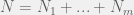
which is just the replicator dynamics. Thus, replicator dynamics perfectly describe an exponentially growing population, at least whenever you are comfortable with using differential equations to model the exponential growth.

Of course, there is still some slight-of-hand going on in this post. I didn’t specify what functional form the many $w_k$ that we encountered have. We often assume that they are simple functions — like lines — of the $x_k$ s, but that need not be the case. Instead, they might be simple functions of density, or ratio (Arditi, & Ginzburg, 1989); or maybe just complicated. If they are not simple functions of the $x_k$ s then solving the dynamics might be unwieldy (although replicator dynamics are already unwieldy to solve), but equilibrium analysis is often still tractable.^[8]

The take home message is that the replicator equation is simple and flexible. This flexibility makes it difficult to dismiss out of hand, or on only theoretical considerations. But this flexibility also forces us to think carefully about how we will realize theoretical terms like fitness and how we would measure games in experiments.

Notes and References

Although this is usually associated with the work of Hilary Putnam and Jerry Fodor from the 60s and 70s, we can see its antecedents in the writings of Alan Turing (1950) a decade prior. He reminds us that there is nothing special about electricity when it comes to computation and the mind:

The fact that Babbage’s Analytical Engine was to be entirely mechanical will help us to rid ourselves of a superstition. Importance is often attached to the fact that modern digital computers are electrical, and that the nervous system also is electrical. Since Babbage’s machine was not electrical, and since all digital computers are in a sense equivalent, we see that this use of electricity cannot be of theoretical importance.
As I’ve discussed previously, evolutionary game theory was born out of statics with Maynard Smith & Price (1973) introducing the concept of an evolutionary stable strategy. Only after did Taylor & Jonker (1978), Hofbauer, Shuster & Sigmund (1979), and Zeeman (1980) give it the dynamic formulation I discuss here.
In other words, the macroscopic statement of the replicator equation can be viewed as an implicit definition of the abstract concept of fitness. This is often forgotten, when people assume that fitness has a single and obvious system-independent definition. See Orr (2009) for a discussion of common confusions over fitness in the literature.
Traulsen et al. (2006) actually achieve a more general result, by starting with a Moran process that also considers mutations between strategies and in the limit of large populations recovering the replicator-mutator equation in Maynard Smith form.
If the Taylor form of the replicator equation is desired then Traulsen et al. (2006) show how to achieve this, too. Instead of birth-death, they consider an imitation process. Two agents are selected uniformly at random, and individual if the payoff of the first individual is $w_1$ and the second is $w_2$ then the first copies the second with probability:

$p = \frac{1}{2} + \frac{s}{2}\frac{w_1 - w_2}{\Delta w}$

where $\Delta w$ is the maximum possible gap in the payoff of two agents in the model. With this version, they get the Taylor form, with the fitness as payoff, again. They are not the first to derive the Taylor form replicator equation from imitation processes. In fact, Schlag (1998) went further by showing that with the proportional imitation rule (only copy those that have higher payoffs, in proportion to how much higher the payoff is), you not only get the Taylor form replicator equation in a large population limit but also that this local update rule is optimal from the individual agent’s perspective in certain social learning settings.
Experimentally, we can’t grow our populations for arbitrary small times because then the noise of our plating, measurement, and of the biology itself will make the signal of growth rates impossible to detect. As such, we have to make an assumption that growth rates for finite but small times would continue to scale down to smaller and smaller times. In the process, we will make a trade-off between error due to dynamics from too big of $\Delta t$ versus error due to noise from too small of $\Delta t$ . In the case of a time-lapse microscopy system finding the optimal trade-off can be done by looking at the power and goodness-of-fit of an exponential model to our data, but this then takes us into a realm equivalent to the next section.
If you prefer logistic over exponential growth then you can still recover replicator dynamics. The trick is to define a fictitious strategy for each carrying capacity that corresponds to the ’empty space’ of that capacity.
See for example, how Archetti (2013) handles non-linear public goods.

Archetti, M. (2013). Evolutionary game theory of growth factor production: implications for tumour heterogeneity and resistance to therapies. British Journal of Cancer, 109(4): 1056-1062.

Arditi, R., & Ginzburg, L. R. (1989). Coupling in predator-prey dynamics: ratio-dependence. Journal of Theoretical Biology, 139(3): 311-326.

Hofbauer, J., Schuster, P., & Sigmund, K. (1979). A note on evolutionary stable strategies and game dynamics. Journal of Theoretical Biology, 81:609-612.

Maynard Smith, J., & Price, G.R. (1973). The logic of animal conflict. Nature, 246, 15-18

Maynard Smith, J. (1982). Evolution and the Theory of Games. Cambridge University Press.

Orr, H.A. (2009). Fitness and its role in evolutionary genetics. Nature Reviews Genetics, 10(8): 531-539.

Taylor, P., & Jonker, L. (1978). Evolutionary stable strategies and game dynamics. Mathematical Biosciences, 40 (1-2), 145-156 DOI: 10.1016/0025-5564(78)90077-9

Traulsen, A., Claussen, J. C., & Hauert, C. (2006). Coevolutionary dynamics in large, but finite populations. Physical Review E, 74(1): 011901.

Turing, A. M. (1950) Computing Machinery and Intelligence. Mind.

Schlag, K. H. (1998). Why imitate, and if so, how?: A boundedly rational approach to multi-armed bandits. Journal of Economic Theory, 78(1): 130-156.

Shnerb, N.M., Louzoun, Y., Bettelheim, E., & Solomon, S. (2000). The importance of being discrete: Life always wins on the surface. Proceedings of the National Academy of Sciences of the USA, 97(19): 10322-4

Zeeman, E.C. (1980). Population dynamics from game theory. In: Nitecki, A., Robinston, C. (Eds), Proceedings of an International Conference of Global Theory of Dynamic Systems. Lecture Notes in Mathematics, 819. Springer, Berlin.

Filed under Analytic, Commentary, Preliminary, Technical Tagged with Alan Turing, fitness ontology, metamodeling, operationalization, philosophy of science, replicator dynamics

About Artem Kaznatcheev
From the Department of Computer Science at Oxford University and Department of Translational Hematology & Oncology Research at Cleveland Clinic, I marvel at the world through algorithmic lenses. My mind is drawn to evolutionary dynamics, theoretical computer science, mathematical oncology, computational learning theory, and philosophy of science. Previously I was at the Department of Integrated Mathematical Oncology at Moffitt Cancer Center, and the School of Computer Science and Department of Psychology at McGill University. In a past life, I worried about quantum queries at the Institute for Quantum Computing and Department of Combinatorics & Optimization at University of Waterloo and as a visitor to the Centre for Quantum Technologies at National University of Singapore. Meander with me on Google+ and Twitter.