mutation | Theory, Evolution, and Games Group

Mutation-bias driving the evolution of mutation rates

March 31, 2016 by Julian Xue 4 Comments

In classic game theory, we are often faced with multiple potential equilibria between which to select with no unequivocal way to choose between these alternatives. If you’ve ever heard Artem justify dynamic approaches, such as evolutionary game theory, then you’ve seen this equilibrium selection problem take center stage. Natural selection has an analogous ‘problem’ of many local fitness peaks. Is the selection between them simply an accidental historical process? Or is there a method to the madness that is independent of the the environment that defines the fitness landscape and that can produce long term evolutionary trends?

Two weeks ago, in my first post of this series, I talked about an idea Wallace Arthur (2004) calls “developmental bias”, where the variation of traits in a population can determine which fitness peak the population evolves to. The idea is that if variation is generated more frequently in a particular direction, then fitness peaks in that direction are more easily discovered. Arthur hypothesized that this mechanism can be responsible for long-term evolutionary trends.

A very similar idea was discovered and called “mutation bias” by Yampolsky & Stoltzfus (2001). The difference between mutation bias and developmental bias is that Yampolsky & Stoltzfus (2001) described the idea in the language of discrete genetics rather than trait-based phenotypic evolution. They also did not invoke developmental biology. The basic mechanism, however, was the same: if a population is confronted with multiple fitness peaks nearby, mutation bias will make particular peaks much more likely.

In this post, I will discuss the Yampolsky & Stoltzfus (2001) “mutation bias”, consider applications of it to the evolution of mutation rates by Gerrish et al. (2007), and discuss how mutation is like and unlike other biological traits.

Evolutionary games in set structured populations

May 8, 2013 by Artem Kaznatcheev 3 Comments

We have previously discussed the importance of population structure in evolutionary game theory, and looked at the Ohtsuki-Nowak transform for analytic studies of games on one of the simplest structures — random regular graphs. However, there is another extremely simple structure to consider: a family of inviscid sets. We can think of each agent as belonging to one or more sets and interacting with everybody that shares a set with them. If there is only one set then we are back to the case on a completely inviscid population. If we associate a set with each edge in a graph and restrict them to have constant size then we have standard evolutionary graph theory. However, it is more natural to allow sets to grow larger if their members have high fitness.

Tarnita et al. (2009) consider a population of $N$ individuals and $M$ sets, where each individual can belong to $K$ of the sets. Strategy and set membership are heritable (with mutation probabilities $u$ and $v$ , respectively), and interactions are only with agents that share a set (if two agents share more than one set then they interact more than once). However, reproduction is inviscid: a random individual is selected to die and everybody competes to replace them with a child. This set-dependent interaction, makes the model equivalent to the earliest models of ethnocentrism, but the model is not equivalent to more modern approaches to ethnocentrism. Since sets cannot reproduce and migration (through mutation) between sets is purely random, the model also cannot capture group selection. However, cooperation for the Prisoners’ dilemma still emerges in this model, if we have:

$\frac{b}{c} \geq \frac{K}{M - K}(\nu + 2) + \frac{M}{M - K}\frac{\nu^2 + 3\nu + 3}{\nu(\nu + 2)}$

Where $\nu = 2Nv$ is the population-scaled set mutation rate, even when this is zero we get cooperation when $\frac{b}{c} \geq \frac{3}{2} + \frac{7K}{2(M - K)}$ . Alternatively, to simplify we can take the limit of $M >> K = 1$ to get:

$\frac{b}{c} \geq 1 + \frac{1}{\nu}(1 + \frac{1}{\nu + 2}) + \frac{\nu + 2}{M}$

If we allow the maximum number of sets ( $M = N$ ) and take the further limit of large populations $N >> 2$ then this becomes a very simple:

$\frac{b}{c} \geq 1 + 2v$

Finally, in the supplementary materials, the authors derive a very nice relationship for evolution of cooperation on arbitrary cooperate-defect games given by a payoff matrix $\begin{pmatrix}1 & U \\ V & 0\end{pmatrix}$ of:

$\sigma \geq V - U$

where $\sigma$ is a structural constant given by:

$\sigma = \frac{1 + \nu + \mu}{3 + \nu + \mu)}\frac{K(\nu^2 + 2\nu + \nu\mu) + M(3 + 2\nu + \mu}{K(\nu^2 + 2\nu + \nu\mu) + M(1 + \mu)}$

Which in the limit of small population-scaled strategy mutation ( $\mu = 0$ ), and $M >> K$ becomes:

$\sigma = 1 + \nu + \frac{\nu(\nu + 1)}{\nu + 3}$

Since the structural constant is always greater than 1, and since we typically care about large $\nu$ , it is more enlightening to look at the reciprocal that in the limit of large $\nu >> 3$ becomes:

$\frac{1}{\sigma - 1} = \frac{1}{2\nu}$

And simplifies the general equation for cooperation to emerge to:

$1 + 2\nu \geq V - U$

Which can be seen as a relaxation of the classic game theory concept of risk-dominance.

Tarnita, C., Antal, T., Ohtsuki, H., & Nowak, M. (2009). Evolutionary dynamics in set structured populations Proceedings of the National Academy of Sciences, 106 (21), 8601-8604 DOI: 10.1073/pnas.0903019106

Filed under Analytic, Reviews, Technical Tagged with ethnocentrism, evolution of cooperation, Martin A. Nowak, mutation, prisoner's dilemma

Evolutionary games in finite inviscid populations

October 22, 2012 by Artem Kaznatcheev 1 Comment

Last week, we saw how to deal with two-strategy games in finite inviscid populations. Unfortunately, two strategy games are not adequate to model many of the interactions we might be interested in. In particular, we cannot use Antal et al. (2009a) to look at bifurcations and finitary/stochastic effects in tag-based models of ethnocentrism, at least not without some subtle tricks. In this post we are going to look at a more general approach for any $n$ -strategy game developed by Antal et al. (2009b). We will apply these tools to look at a new problem for the paper, but an old problem for the blog: ethnocentrism.

Antal et al. (2009b) consider a large but finite population of size $N$ and a game $A$ with $n$ strategies. For update rule, they focus on the frequency dependent Moran process, although their results also hold for Wright-Fisher, and pairwise comparison (Fermi rule). Unlike the previous results for two-strategy games, the present work is applicable only in the limit of weak selection. Mutations are assumed to be uniform with probability $u$ : a mutant is any one of the $n$ strategies with equal probabilities. However, in section 4.2, the authors provide a cute argument for approximating non-uniform but parent-independent mutation rates by repeating strategies in proportion to the likelihood of mutation into them. Much like the two-strategy case, the authors derive separate equations for low and high mutation rates, and then provide a way to interpolate between the two extremes for intermediate mutation rates.

The mathematics proceeds through a perturbation analysis. The basic idea is to solve for the distribution of strategies in the drift (no selection) model, and then to gradually dial up the selection to perturb the distribution slightly into the weak selection regime. The authors use this to arrive at the following to conditions for low, and high mutation for strategy $k$ to be favored:

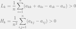
$\begin{aligned} L_k & = \frac{1}{n}\sum_{i = 1}^{n}(a_{kk} + a_{ki} - a_{ik} - a_{ii}) > 0 \\ H_k & = \frac{1}{n^2}\sum_{i,j = 1}^n(a_{kj} - a_{ij}) > 0 \end{aligned}$

There is an intuitive story to help understand these two conditions. In the case of low mutation, the population is usually just two strategies until one of them fixes. So for $L_k$ the terms that matter are the pairwise interactions between the strategies, and since the most decisive (and entropy rich) case is near the 50-50 split in the two strategies, self interactions ( $a_{kk}$ ) and other-strategy interactions ( $a_{ki}$ ) happen with the same frequency. I think this is where the discrepancy with Antal et. al (2009a) that we will see later sneaks in. A correction factor of $\frac{N - 2}{N}$ should be added in front of the the self-interaction terms, but I digress.

For the high mutation case, all the strategies are present in the population with about the same frequency at the same time. We need to look at the transitions from this population to get our first order terms. In that case, the focal individual’s fitness is $f_k = \frac{1}{n} \sum_{j = 1}^n a_{kj}$ (since all opponents are equally likely; once again, I believe a correction term is in order), and the average fitness is $\frac{1}{n} \sum_{i = 1}^n f_i$ . The difference of these two terms produces $H_k$ .

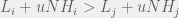
In order to interpolate, we have the following condition for strategy $i$ to be more common than $j$ for intermediate mutation rates $u$ :

$L_i + uNH_i > L_j + uNH_j$

How does this disagree with the two-strategy results of Antal et al. (2009a)? The present paper reproduces the condition of risk-dominance, with C dominating D if $1 > V - U$ , but does not produce the small $N$ correction of $\frac{N - 2}{N} > V - U$ . This would be mitigated with the observations I made earlier, but the approach of the perturbation analysis would have to be modified carefully.

The perturbation method can be extended to mixed strategies, as is done by Tarnita et al. (2009). In that case, we just replace the summation by integrals, to get:

$\begin{aligned} L_p & = \frac{1}{||S_n||}\int_{S_n}(p^TAp + p^TAq - q^TAp - q^TAq) dq > 0 \\ H_p & = \frac{1}{||S_n||^2}\int_{S_n} \int_{S_n} (p^TAq - r^TAq) dq dr > 0 \end{aligned}$

Where $S_n$ is the n-vertex simplex with volume $||S_n|| = \frac{\sqrt{n}}{(n - 1)!}$ . It is nice to know that the results generalize to mixed strategies, but not as important tool as the pure strategy variant. I will concentrate on pure strategies, although mixed might be good to revisit to study evolution of agency.

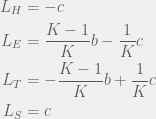
Antal et al. (2009b) showcase their method with three case studies: (i) cooperators, defectors, and loners, (ii) reversing the rank of strategies by mutation, and (iii) cooperators, defectors, and tit-for-tat. The first is the most interesting for me, since it shows how adding an irrelevant strategy, can reverse the dominance of the other two. I will present their example in a more general context for all cooperate-defect games. We will introduce an irrelevant strategy L, where irrelevance means that both C and D get the same payoff $X$ from interacting with L and L gets $Y$ from them. The self interaction payoff for L can differ, and we can set it to $Z$ :

$\begin{pmatrix} 1 & U & X \\ V & 0 & X \\ Y & Y & Z \end{pmatrix}$

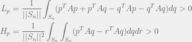
The authors consider the particular case of $V = 9/8$ and $U = -1/8$ , and $X = Y = Z = -1/4$ . We can apply the general results to get (for small mutations):

$\begin{aligned} L_C & = \frac{1}{3}(2 + U - V + X - Y - Z) \\ L_D & = \frac{1}{3}(V - U - 1 + X - Y - Z) \\ L_L & = \frac{1}{3}(2(Y - Z) - 1) \end{aligned}$

We can look at at the condition for C to dominate D for small mutations ( $L_C > L_C$ ) to get $\frac{3}{2} > V - U$ . If we had used $M$ different irrelevant strategies (or just dialed up the proportion of mutations to an irrelevant strategy) then $\frac{3}{2}$ would be replaced by $1 + \frac{M}{2}$ . This creates a new strip of cooperation which reaches into the Prisoner’s dilemma region (drawn in blue):

When we switch to large mutations, the region disappears and we recover the standard $1 > V - U$ rule. Note that this example means that, for this analysis, we cannot ignore competing strategies even if they are strictly dominated.

Ethnocentrism in tag-based models

We will consider a strategy space of $K$ tags, with an agent of each tag being either a humanitarian (cooperate with all), ethnocentric (cooperate with same-tag), traitorous (cooperate with oot-tags), or selfish. For the game, we will look at the usual cost-benefit representation of Prisoner’s dilemma. Note that the $L$ and $H$ values will be the withing a single strategy of different tags, so we only need to compute four of each:

$\begin{aligned} L_{H} & = -c \\ L_{E} & = \frac{K - 1}{K}b - \frac{1}{K}c \\ L_{T} & = -\frac{K - 1}{K}b + \frac{1}{K}c \\ L_{S} & = c \end{aligned}$

This divides the dynamics into two regions, when $\frac{K - 1}{K + 1} > \frac{c}{b}$ then $E > S > H > T$ , otherwise we have $S > E > T > H$ . In other words, for large enough $K$ or small enough $c/b$ , ethnocentrism can be the dominant strategy in the population. This condition is in perfect agreement with the Traulsen & Nowak (2007) results we saw earlier. Although in that case, there were no H or T agents. If we remove H & T from the current analysis, we will still get the same condition for ethnocentric dominance even though we will calculate different $L$ values.

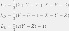
For large mutations, the advantage of ethnocentrics disappears completely, and we get:

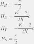
$\begin{aligned} H_{H} & = -\frac{c}{2} \\ H_{E} & = \frac{K - 2}{2K}c \\ H_{T} & = -\frac{K - 2}{2K}c \\ H_{S} & = \frac{c}{2} \end{aligned}$

Which for $K \geq 2$ results in the ordering 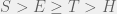$S > E \geq T > H$ . So if we have mutations that change tag and strategy together (as they do in this case) then higher mutation rates disadvantage the population, and if we let $M = uN$ be the expected number of mutants per generation, then we can see that ethnocentric cooperation is possible only if $M < (K - 1)\frac{b}{c} - (K + 1)$ or rewritten as $\frac{K - 1}{M + K + 1} > \frac{c}{b}$ .

References

Antal, T., Nowak, M.A., & Traulsen, A. (2009a). Strategy abundance in games for arbitrary mutation rates Journal of Theoretical Biology, 257 (2), 340-344.

Antal T, Traulsen A, Ohtsuki H, Tarnita CE, & Nowak MA (2009b). Mutation-selection equilibrium in games with multiple strategies. Journal of Theoretical Biology, 258 (4), 614-22 PMID: 19248791

Tarnita, C.E., Antal, T., Nowak, M.A. (2009) Mutation-selection equilibrium in games with mixed strategies. Journal of Theoretical Biology 26(1): 50-57.

Traulsen A, & Nowak MA (2007). Chromodynamics of cooperation in finite populations. PLoS One, 2 (3).

Filed under Analytic, Reviews, Technical Tagged with discrete vs continuous, ethnocentrism, Martin A. Nowak, mutation, prisoner's dilemma

Risk-dominance and a general evolutionary rule in finite populations

October 18, 2012 by Artem Kaznatcheev 5 Comments

In coordination games, the players have to choose between two possible strategies, and their goal is to coordinate their choice without communication. In a classic game theory setting, coordination games are the prototypical setting for discussing the problem of equilibrium selection: if a game has more than one equilibrium then how do the players know which one to equilibrate on? The standard solution concept for this is the idea of a risk dominance. If you were playing a symmetric coordination game:

$\begin{pmatrix}R & S \\ T & P \end{pmatrix}$

where $R > T$ and $P > S$ , then how would you chose your strategy not knowing what your opponent is going to do? Since the two pure strategy Nash equilibria are the top left and bottom right corner, you would know that you want to end up coordinating with your partner. However, given no means to do so, you could assume that your partner is going to pick one of the two strategies at random. In this case, you would want to maximize your expected payoff. Assuming that each strategy of your parner is equally probably, simple arithmetic would lead you to conclude that you should chose the first strategy (first row, call it C) given the condition:

$R + S > T + P$

Congratulations, through your reasoning you have arrived at the idea of a risk dominant strategy. If the above equation is satisfied then C is risk dominant over D (the second strategy choice), more likely to be selected, and the ‘better’ Nash equilibrium.

Since many view evolutionary game theory as a study of equilibrium selection, it is not surprising to see risk-dominance appear in evolution. In particular, if the risk dominance condition is met, then (for a coordination game and replicator dynamics) C will have a larger basin of attraction than D. If we pick initial levels of cooperators at random, then in your well-mixed and extremely large population, the risk-dominant strategy will dominate the population more often. If you are feeling adventurous, then I recommend as exercise to calculate the exact probability of C dominating in this setting.

From our experience with ethnocentrism and discrete populations, we know that replicator dynamics is not the end of the story. The second step is to consider finite inviscid populations where we can’t ignore dynamical stochasticity. Kandari et al. (1993) studies this setting and for a population of size $N$ concluded that C would be a more likely than D if:

$R(N - 2) + SN > TN + P(N - 2)$

Nowak et al. (2004) looked at this problem from the biological perspective of Moran processes. In a Moran process, there is no mutation, and thus the conclusion of dynamics is the absorbing state of either all C or all D. The quantity of interest becomes the fixation probability: the fixation probability of C is the probability that a single C mutant invades (leads to an all C absorbing state) a population of all D (vice-virsa for
fixation of D). Nowak et al. (2004) found that the fixation probability of C (in the weak selection limit) is higher than that of D in a population of $N$ agents if and only if the above equation is satisfied.

Antal et al. (2009) concluded this research program. They showed that the above condition was necessary for the case of arbitrary mutations, a wide range of evolutionary processes, and any two player, two strategy game. It is true for pair-comparison (Fermi rule), exponential Moran processes, and weak-selection Moral processes with arbitrary mutation rates. In general, any update process that satisfies the two requirements: (i) additive payoffs, and (ii) evolutionary dynamics depend only on the payoff differences.

Let us visualize this result. As we learnt in a previous post we know that a two strategy cooperate-defect games do not need 4 parameters to specify, and can be rewritten with just two. The symmetry arguments we applied before preserve the authors’ result, so let’s apply the transformation:

$\begin{pmatrix}R & S \\ T & P \end{pmatrix} \Rightarrow \begin{pmatrix}1 & U \\ V & 0 \end{pmatrix}$

This lets us simplify the risk-dominance and finite population rules to:

$1 > V - U \quad \text{and} \quad \frac{N - 2}{N} > V - U$

Now it clear why we discussed risk-dominance before diving into finite populations. As the population size gets arbitrarily large ( $N \rightarrow \infty$ ), our finite population rule reduces to risk-dominance and replicator dynamics. In the other extreme case is $N = 2$ (can’t have a game with smaller populations) the rule becomes $U > V$ .

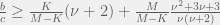
In the above picture of U-V space, we can see the two extreme conditions. In the green region, C is more likely than D for any population size, and in the blue it is true in the limit of infinite population. For particular $N > 2$ you get a different division line in the blue region parallel to the two current ones. Give a specific game in the blue region, you can calculate the threshold:

$N^* = \frac{2}{1 - (V - U)}$

For games in the blue region, if your population exceeds the $N^*$ threshold then C with be more likely than D.

For those interested in the mathematical details, I recommend sections 2.3 and 4 of Antal et al. (2009). In particular, I enjoy their approach in section 2.3 of showing that when the game is on the dividing line then we have a symmetric distribution around $N/2$ and due to the well-behaved nature of deformations of the game matrix we can extend to the non knife-edge case. The only missing study in Antal et al. (2009) is a study of the second moment of the population. In regions 5, 9, and 10 we expect a bimodal distribution, and in 2-4 and 6-8 a unimodal. Can we use the probability of mutation to bound the distance between the peaks in the former, and the variance of the peak in the latter? Another exercise for the highly enthusiastic reader.

References

Antal, T., Nowak, M.A., & Traulsen, A. (2009). Strategy abundance in games for arbitrary mutation rates Journal of Theoretical Biology, 257 (2), 340-344 DOI: 10.1016/j.jtbi.2008.11.023

Kandori, M., Mailath, G.J., & Rob, R. (1993). Learning, mutation, and long run equilibria in games. Econometrica 61(1): 29-56.

Nowak, M.A., Sasak, A., Taylor, C., & Fudenberg, D. (2004). Emergence of cooperation and evolutionary stability in finite populations. Nature 428: 646-650.

Filed under Analytic, Reviews, Technical Tagged with classic game theory, discrete vs continuous, Martin A. Nowak, mutation

Critique of Chaitin’s algorithmic mutation

July 8, 2012 by Artem Kaznatcheev 4 Comments

Last week, I reviewed Gregory Chaitin’s Proving Darwin. I concentrated on a broad overview of the book and metabiology, and did not touch on the mathematical details; This post will start touching. The goal is to summarize Chaitin’s ideas more rigorously and to address Chaitin’s comment:

I disagree with your characterization of algorithmic mutations as directed.
They are in fact random.
Rgds,
GJC

Specifically, I need to (a) summarize the mathematical details of algorithmic mutations, (b) clarify the distinction between random mutation and (what I called) randomized directed mutation, and (c) defend my assertion that algorithmic mutations are not purely random but directed. I need to fully explain my earlier claim:

The algorithmic mutation actually combine the act of mutating and selecting into one step, it is a $n$ -bit program that takes the current organism A and outputs a new organism B of higher fitness (note, that it needs an oracle call for the Halting-problem to do so). The probability that A is replaced by B is then $2^{-n}$ . There is no way to decouple the selection step from the mutation step in an algorithmic mutation, although this is not clear without the technical details which I will postpone until a future post. Chaitin’s model does not have random mutations, it has randomized directed mutations.

The high level description of algorithmic mutations given in Chapter 5 is not necessarily inconsistent with random mutations, but it is not detailed enough to make a concrete judgement. We have to look at Appendix 2 (The Heart of the Proof) to really understand how Chaitin’s mutations act. As before, an organism $A$ is a halting self-delimiting program, and $A$ ‘s fitness $\phi(A)$ is the integer $A$ outputs upon halting. I will use $t(A)$ to mean the running time of $A$ and will set $t(P) = \infty$ for a non-halting program $P$ .

A mutation $M_K$ works as follows. $M_K(A)$ calculates a lowerbound $\Omega_{\phi(A)} = \sum_{A \in S(\phi(A))} \frac{1}{2^{|A|}}$ of Chaitin’s constant $\Omega$ , where $S(N)$ is the set of programs smaller than $N$ bits in length and halting by $N$ steps. $M_K$ calculates a new number $\beta = \Omega_{\phi(A)} + 2^{-K}$ and mutates $A$ into $A' = \pi\beta$ . Here $\pi$ is a self-delimiting prefix that finds the first $N$ such that $\Omega_N \geq \beta$ , outputs $N$ , and halts. If $\beta < \Omega$ then $A'$ a halts and is thus an organism with fitness $\phi(A') = \beta$ . If $\beta \geq \Omega$ then $A'$ is a non-halting program and thus not an organism (or at best an organism with an undefined fitness $\phi(A')$ ). Chaitin’s mutations either return a strictly more fit organism, or do not return one at all (equivalently: an organism with undefined fitness).

To simulate evolution (as opposed to a deterministic picking of mutations), Chaitin selects the mutations randomly (with mutation $M_K$ being selected in proportion to $2^{-|M_K|}$ ). This is probably why he writes them as ‘random’, however picking a directed mutation at random, is just randomized directed mutation. The concept of a mutant having lower fitness, is undefined in metabiology. A defense would be to say that algorithmic mutations actually combine the steps of mutation and selection into one — this is a technique that is often used in macroevolutionary models. However, I cannot grant this defense, because in macroevolutionary models, even when a fitter agent is always selected, the mutations are still capable of defining an unfit individual. Further, when macroevolutionary models set up such a hard gradient (of always selecting the fitter mutant) then these models are not used to study fitness because it is trivial to show unbounded fitness growth in such models.

Is Chaitin’s model the simplest it can be? Chaitin spends the first four chapters defending algorithms/software as metaphors for genes; Does metabiology actually use the power of algorithms? Chaitin does not attempt to address abiogenesis in his model and the first organism is an arbitrary program. Every subsequent program arises from the original by a sequence of algorithmic mutations; but every mutation returns an program of the form $\pi \beta$ where $\beta$ is some rational number greater than 0 and less than $\Omega$ . In other words, the genes are only capable of programming:

N = 1
while $\Omega_N < \beta$ do N = N + 1 end
print N

I hid the subroutine that computes $\Omega_N$ but we will see that it is a superficial feature. $\beta$ and the N that the algorithm returns are completely equivalent. A larger $\beta$ returns a larger N. Since the prefix $\pi$ is always repeated, I will just represent organisms by the rational number after $\pi$ . Instead of $\pi \beta$ , I will write $\beta$ . Now, I can simple re-define the fitness function:

$\phi(\beta) = \begin{cases} \beta & \mathrm{if} \; \beta < \Omega \\ \bot & \mathrm{otherwise} \end{cases}$

and the mutation operator:

$M_K(\beta) = \begin{cases} \beta + \frac{1}{2^K} & \mathrm{if} \; \beta < \Omega - \frac{1}{2^K} \\ \beta & \mathrm{otherwise} \end{cases}$

and metabiology remains completely unchanged, with the exception of the original organism which we can just set as 0 for our purposes. Of course, instead of the fitness growing higher and higher it grows to be a better and better lower bound for $\Omega$ . All the algorithms are stripped away, except in that $\Omega$ comes from algorithmic information theory. However, we don’t need $\Omega$ to achieve all of Chaitin’s results: we can use any irrational number between 0 and 1 like $\frac{1}{\sqrt{2}}$ (in fact, the number doesn’t even need to be irrational it just has to have a non-terminating expansion in base 2). In other words, the algorithmic part of metabiology is superficial.

Further, by looking at metabiology in the simple terms I described above we can also overcome the directed nature of ‘algorithmic’ mutations. We just modify the mutation operator to be indexed by K and either – or + with both K and – or + selected from some distribution. A natural distribution is to pick K proportional to $2^{-K}$ and – or + uniformly. Now, we can define a random mutation operator:

$M_{K,+} \begin{cases} \beta + \frac{1}{2^K} & \mathrm{if} \; \beta < \Omega + \frac{1}{2^K} \\ \beta & \mathrm{otherwise} \end{cases}$

and

$M_{K,-} \begin{cases} \beta - \frac{1}{2^K} & \mathrm{if} \; \beta \geq \frac{1}{2^K} \\ \beta & \mathrm{otherwise} \end{cases}$

Then given a focal organism $\beta$ and a mutant $\beta'$ we can use our favorite selection rule to chose who survives. A tempting one is to use Chaitin’s hard-max and let whoever is larger survive. Alternatively, we can use a softer rule like $\beta'$ takes over with probability proportional to $exp(\beta' - \beta)$ (this is a popular rule in evolutionary game theory models). Alternatively, we can stick ourselves plainly inside neutral evolution and just say $\beta'$ always takes over regardless of fitness. This would create a random walk model, which can still show an increase in complexity as proposed by Gould (1997) and summarized on this blog by Julian.