Drug holidays and losing resistance with replicator dynamics
September 2, 2016 7 Comments
A couple of weeks ago, before we all left Tampa, Pranav Warman, David Basanta and I frantically worked on refinements of our model of prostate cancer in the bone. One of the things that David and Pranav hoped to see from the model was conditions under which adaptive therapy (or just treatment interrupted with non-treatment holidays) performs better than solid blocks of treatment. As we struggled to find parameters that might achieve this result, my frustration drove me to embrace the advice of George Pólya: “If you can’t solve a problem, then there is an easier problem you can solve: find it.”
 In this case, I opted to remove all mentions of the bone and cancer. Instead, I asked a simpler but more abstract question: what qualitative features must a minimal model of the evolution of resistance have in order for drug holidays to be superior to a single treatment block? In this post, I want to set up this question precisely, show why drug holidays are difficult in evolutionary models, and propose a feature that makes drug holidays viable. If you find this topic exciting then you should consider registering for the 6th annual Integrated Mathematical Oncology workshop at the Moffitt Cancer Center.[1] This year’s theme is drug resistance.
Discontinuous treatment powered by holidays
Most discussions of treatment holidays are focused on managing toxicity. Especially in the case of chemotherapy, the treatment is often devastating to the patient. For many therapies, the limiting factor is for how long (or how strong) a patient can be treated without being killed by the therapy. Thus, these holidays aren’t the active ingredient of the therapy, they are not what lets the therapy supress cancer cells. These holidays are a way to manage side-effects. And although I think it can be very important to focus on the toxicity of treatment, in this case I want to think about the case where holidays are a central driver behind the effectiveness of therapy. Is there a class of therapies and evolutionary dynamics such that the drug fails to treat the tumour unless its application is interspersed with holidays of no treatment?
In particular, I want to consider two therapies of the same strength (per unit time) that have the same start and end time. The continuous case would run continuous treatment from the start time to the end time. The discontinuous therapy punctuates blocks of treatments with holidays from the start time until the end time. Thus, I want to consider cases where the discontinuous therapy has strictly less therapy. And yet, I want to find settings under which the tumour burden at the end time is lower for the discontinuous therapy.
Minimal model and the difficulty of discontinuous treatment
Of course, in a real clinical setting, we might not care if a discontinuous treatment works by allowing a different dosage, recovery of sensitivity, or booting up the patient’s immune system. We only really care that it works. But if we consider all three (or more) effects at once in a heuristic model — or in a big simulation — then we won’t really understand why our strategy succeeds. Thus, in this post, I want to isolate just the recovery-of-sensitivity-during-treatment-holidays aspect of the strategy.
I will start with one of the simplest possible model of resistance. A tumour (or pathogen) growing towards carrying capacity. There is a single therapy and two tumour subtypes: a sensitive type of density 


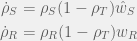
where 


Unfortunately, under these conditions, it is clear that 


Resensitization of the resistant population
To overcome this, we need a way for 
There are several ways we could interpret these equations, but my favourite option is to think of them as individual cells losing resistance. When under stress, each resistant cell re-evaluates its commitment to investing energy in resistance and gives up that strategy at a rate of 


When treatment is on, the resistant proportion will grow back but it is possible to still have the total tumour burden shrink by killing sensitive cells quickly enough. In order for total tumour volume to shrink, we need 


Unfortunately, just those conditions are not enough to guarantee that discontinuous therapies can control the tumour burden and outperform a single continuous treatment. The rates of loss of sensitivity under treatment and growth of tumour burden without treatment have to be low enough to be surpassed by the rate of loss of resistant density without treatment and loss of tumour density with treatment. It is probably possible to calculate these rates analytically and also solve for the average burden of the controlled tumour. However, this was meant to be a quick post so I only present a proof of concept by simulation.3
Proof of concept and adaptive therapy
Below is a figure showing an example of when discontinuous therapy outperforms a continuous therapy of equal strength. All parameters — except the times that treatment is turned on or off — are the same across the two simulations of the ODEs. These parameters are: 


In the top panel with a continuous therapy, as expected, the resistant population quickly takes over the whole tumour, grows the tumour to carrying capacity, and leaves the patient with a tumour burden of 1. With discontinuous treatment, it is possible to time treatment holidays such that the resistant tumour burden is kept oscillating around ~0.3 and the total tumour burden is kept oscillating around ~0.85 without ever surpassing ~0.93. This is not a huge reduction in tumour burden but it does show how holidays can help us control a tumour that is unresponsive to continuous therapy.
If you are curious, the discontinuous treatments in the second panel are from times 1 to 2, 3.5 to 4.5, 6 to 9, 10 ti 13, 14 to 17.5, 18.5 to 22.5, 23.5 to 27, 28 to 32, and 33 to 35. While the continuous treatment is just a single block from 1 to 35. In other words, the discontinuous treatment includes a total of 9 time-steps of holidays distributed over eight holidays (the first two are 1.5 time-steps long while the rest are 1). Thus, the discontinuous treatment produces a better outcome even though it ends up applying less than 74% of the drug-hours of the continuous treatment.
In this example, I tuned the treatment timings by eye but it is not hard to adapt my strategy into an adaptive therapy. A theoretical route might be to pick up upper sensitivity threshold 


The practical route is a pretty obvious strategy for adaptive therapy. And I wouldn’t be surprised if doctors do something like this already. Although usually, they switch to a new drug when a tumour stops responding to an existing one. Thus, the difficulty becomes characterising the sort of tumours (or evolutionary dynamics) for which this discontinuous strategy will outperform a continuous counterpart. Then we can know when to return to and old drug to achieve tumour control instead of switching to a new drug in the hopes of a cure.
Notes
- Whether you work in mathematical oncology or in more general modeling of biological systems then I recommend this event. I have attended for the past three years and plan to attend this year. I greatly enjoyed each prior year: 2013, 2014, 2015. Here is a video of the 3rd workshop to whet your appetite:
-
Note that the structural feature of fitness-based growth rate depending on
- I would prefer to not succumb to the curse of computing and avoid relying on ad hoc examples of parameters from simulations. From playing with simulations, it looks like the result is robust. However, for the parameters I tried, the average burden of the controlled tumour is still uncomfortably high. It seems that each parameter setting has an associated region of control, but I cannot figure out how tweaks to the parameters exactly affect the average controlled burden. An analytic treatment would help me resolve this. Unfortunately, I can only come up with rough analytic approximations by discretizing the cycles into two steps. This is not unreasonable — especially since under log or logit transform the ‘waves’ look close to piecewise linear — but not perfect. If you have ideas on a more grounded analytic treatment, dear reader, then let me know. I will also play around on my own when I have time and report back with any successes.


Your \mu parameter, which is not dependent on fitness or environmentally modulated, is precisely the definition of bet-hedging in the ecological sense. There’s a good mathematical theory of how the population fitness (your w_T) is related to the statistics of a stochastically fluctuating or cyclic environment. For example, this paper by Muller: http://dx.doi.org/10.1016/j.jtbi.2013.07.017. Most theoretical studies focus on values of \mu that maximise fitness for a certain fluctuating environment. The reverse problem, which you’re describing here, should be approachable using the same methods.
It should be noted that although your post begins with a discussion of evolutionary modelling, there is actually no evolution occurring in your model. Instead, you have simulated the dynamics of a single bet-hedging strategy (defined by \mu) under two regimes of environmental dynamics. The control you find with metronomic therapy will not be sustainable (for many parameter sets) if you permit \mu to change through evolution and maximise the expected population fitness. This failure of therapy, driven by a change in the proportion of phenotypes as opposed to the emergence of a novel resistant phenotype, would be much more difficult to identify experimentally. However, if metronomic therapy is to become widespread we should pay close attention to whether such a mechanism of resistance does arise.
Finally, there are non-evolutionary mechanisms that might cause treatment holidays to be effective. For example, Mark Roberston-Tessi showed that the interaction between the spatial constraint of aggressive phenotypes and drug–induced cell death can favour metronomic therapies over continuous doses (http://europepmc.org/articles/pmc4421891).
Thanks for the comment, Dan. Some responses:
Good observation. Looking at treatment on/off as switching between different environments and your thoughts about bet hedging were definitely a motivator for this post. Unfortunately, I don’t think this is completely bet-hedging, since it is environmentally modulated. Although I might not have made that explicit enough in my writing. i.e. when treatment is on, there is no . Or maybe to be more consistent with my other terminology:
  . If strategy switching was allowed under treatment then in the top figure we would not have the resistant population saturate to maximal tumour burden.
I think that my most direct inspiration for the switch-when-not-stressed view was the way Andriy Marusyk talked about cells losing resistance in our time lapse experiments. Although this post was not meant to have anything to do with that experiment, I think that Andrew Dhawan is starting to look at this connection more carefully.
I will check out the Muller et al. paper you linked. I think that you’ve sent it to me before and I’ve constantly been putting off reading it carefully.
I completely agree. If I was naming replicator dynamics today, I would call it “ecological game theory” or “ecological dynamics” (as people named correctly for Lotka-Volterra). Unfortunately, the name of evolutionary dynamics for non-innovative replicator dynamics has been entrenched already, and the term of ecological games is being used for something else (which this post would also fall under, since I am looking at densities, not proportions).
And if I allow any of the other parameters ( , etc) to evolve then cancer will also escape all treatments since that maximises its fitness. That is why none of the parameters are evolving since I am assuming they are based on some sort of restrictions from the underlying circuitry of the healthy cell that is being hijacked. In other words, I am considering a world where there are only two viable (pheno)types: S and R and then looking at the population dynamics. Where the rate
  is part of the definition of the R phenotype.
This is a very good point.
This is a pretty cool mechanism, I think it is the one that David Basanta prefers, too. Looking at spatial effects on population dynamics is important. Once I figure out how to operationalize spacial structure to my satisfaction, I will try to think about this angle, too.
Pingback: Don’t take Pokemon Go for dead: a model of product growth | Theory, Evolution, and Games Group
Great post @kaznatcheev! Some ideas: could be a cool extension to consider plasticity into a state of collateral sensitivity. Perhaps leading to interesting regimens of 2 interspersed drugs to minimize resistance?
Also, realizing more and more from experimental data that cell cycle effects here are quite important – quiescence can happen during chemo – this might affect rate of resistance arising, and if planning treatment regimens where things change on the order of days, these effects become non-negligible for modelling. Further, cells may take time to “compute” solutions to the problem of resistance, but once this is done, the rate at which it occurs changes greatly, and the ‘cost’/persistence of this remains to be experimentally determined – should consider this effect as well in the dynamics.
Pingback: Dark selection and ruxolitinib resistance in myeloid neoplasms | Theory, Evolution, and Games Group
Pingback: Cataloging a year of cancer blogging: double goods, measuring games & resistance | Theory, Evolution, and Games Group
Pingback: Local peaks and clinical resistance at negative cost | Theory, Evolution, and Games Group