May | 2012 | Theory, Evolution, and Games Group

Basic model of citation network dynamics

May 13, 2012 by Artem Kaznatcheev 1 Comment

This is a note based on a May 17, 2010 discussion with Julian Z. Xue outlining some of the basic ideas behind a model for citation networks and their dynamics. Inherent in our model, is the need to study dynamics of citation networks over time. How do papers accumulate citations? How do researchers decide which papers to read? What publishing strategies do they use? How much of their attention is devoted to new papers, and how much to well established ones? This already provides us a basic model of actors and the dynamic domain.

The actors: scientists

The actors in our model, are the `scientist’ entities that decide on how to allocate their time between the myriad papers they could read, and decide when they have read enough to publish a paper based on the insights they gained. Associated with each scientist $S$ is a set $F(S)$ corresponding to the folder of papers the scientist has already read.

The dynamic domain, however, is not the scientists, but the papers and citations. Although we might eventually explore the dynamics of which scientists perform better (evolutionary dynamics), or how individual scientists might optimize their own impact (local Hill-Climbing), the starting point can be a fixed distribution of scientist and what kind of network of papers such a distribution produces.

The dynamic domain: the paper-citation network

The primary dynamic domain is the papers and the citation network between them. We will represent this network as a directed acyclic graph (lets keep references of `in press’ works – and the potential cause of cycles – out of this for now) $G(V,E)$ . Each vertex $v \in V$ is a paper and has associated with it two values:

$A(v)$ is the awesomeness of $v$ . This might not be the most technical term, but it is suppose to capture the basic inherent quality of a paper. Sure, the impact of a paper might be influenced by how fashionable the topic is, how well known the author is, and chance occurrences. However, there is still some inherent “awesomeness” to a quality paper, usually in the form of technical merit, soundness, clarity, and novelty of ideas (of course, novelty is inherently time-dependent, and we will return to that). This parameter is private.
$T(v)$ is the age of $v$ (or alternatively, and easier for computational models, the time it was published). For now, I will keep it as age, for my convenience, and so it will start at $0$ and increment by $1$ at each time step. There are two reasons we want to track age: (1) this is suppose to be a dynamic model, we need a time parameter, and (2) we want the novelty of papers to disappear with time. This parameter is public.

The parameters $A(v)$ and $T(v)$ will interact to produce some time dependent value $U(v)$ of a paper. In general, we want $U(v) = A(v)$ when $T(v) = 0$ and to decrease monotonically as the paper ages. A simple candidate is exponential decay, or in more economics/AI friendly terms — discounting:

$U(v) = \alpha^{T(v)} A(v)$

Where $0 < \alpha < 1$ . At this point, $\alpha$ is our only real time scale, apart from the discretization caused by $T(v) \in \mathbb{N}$ we would encounter in a computational formalization. Hence, we cannot expect anything crazy to come from it. This is a bit disappointing since an obvious difference between fields like life science and math is this discounting factor. To analyze such differences, we will need a second time scale to cause conflict, but I am sure that can be arranged.

The dynamics: publications

At each time step, an agent $S$ can query any number of papers (all of them if he so desires) for two public parameters: $T(v)$ and $d_{\mathrm{in}}(v)$ . Where $d_{\mathrm{in}}(v)$ is simply the number of incoming edges to $v$ from elsewhere in $G$ (we might also want to allow access to $d_{\mathrm{out}}$ , but for now that will only complicate things). After sampling the papers, the agent can pick one paper $v$ (that is not already in $F(S)$ ) and learn it’s private awesomeness value $A(v)$ and thus conclude $U(v)$ . This is an analogy to a scientist carefully reading a paper and learning the tricks and merits presented in the paper at a level she can use in future work. At this point, she can add the tuple $(v,0)$ to her folder $F(S)$ of papers. The second part of the tuple is an integer, corresponding to how many times $S$ has used the mentioned paper in her publications.

New publications

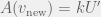
Once an agent $S$ has enough quality original research in his folder, he can publish a new result based on these findings. Since there is some minimal peer review around, there is some minimal threshold of awesomeness $U_{\mathrm{min}}$ that the collection must surpass (in a more complicated model we can consider several journals with different values of $U_{\mathrm{min}}$ , but for now we will stick to a field-wide value). In particular, if a scientist has acquired a subset $R \subseteq F(S)$ and it clears the minimal criterion of awesomeness:

$\Sigma(R) = \sum_{(v,n) \in R} \beta^n U(v) \geq U_{\mathrm{min}}$

then the scientist can use $R$ as the set of references for his publication $v_{\mathrm{new}}$ . Note that the above equation discounts the awesomeness of each paper you are reusing by a factor of $0 < \beta \leq 1$ for each time you have used the paper in your folder before. This is on top of the decay the paper already received to $U(v)$ from time passage. This allows a researcher to re-cite a paper without abusing that privilege. If the scientist decides that he wants to use subset $R$ as the reference list for his new paper, then he melds the ideas in his mind to produce a new paper $v_{\mathrm{new}}$ . In the process, for each $(v,n) \in R$ we replace $(v,n) \in F(S)$ by $(v,n+1)$ . Then, we calculate the awesomeness of the new paper. For this, we first find the mean of the current awesomeness of the citation list:

$\langle U \rangle = \frac{1}{|R|}\sum_{(v,n) \in R} U(v)$

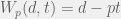
Note that in the above case we do not discount the mean awesomeness by the researchers reuse of the paper. Although the paper cannot spark the same amount of new ideas needed for the researcher who used it (to clear the min threshold), for other researchers, $U(v)$ is still the accurate value of paper $v$ and hence can be used in the average. Then, from a fixed distribution $\mathbb{U}$ with mean $\langle U \rangle$ we sample a value $U'$ . An from this we achieve the awesomeness of the new paper:

$A(v_{\mathrm{new}}) = kU'$

Where $k$ is a positive constant. In general, we will need $k > \alpha^{-m}$ where $m$ is the average time between publications from an individual scientist. Otherwise our system will spiral out of control with constantly decreasing values of $A$ for new papers, eventually making it impossible to clear the $U_{\mathrm{min}}$ threshold. In general $k$ might depend on the individual scientist, but since we are not studying individual scientist in this simplest model, we might as well assume that $k$ depends on the field.

The last important factor is to chose a distribution $\mathbb{U}$ . We need some important properties from this distribution:

$\mathbb{U}$ cannot have support on negative values. It doesn’t really make sense to have negative value for papers. I guess in a completely pessimistic world it is possible to produce papers of negative value, but it doesn’t seem to make sense in our model since a negative value paper would never be cited
or included in any other paper. For simplicity I think we should assume $U \geq 0$ .
$\mathbb{U}$ must be relatively well behaved, especially if we want to have an analytic treatment. For an analytic treatment in particular, it might be smart to keep the distribution as unspecified as possible until the latest possible moment in the analysis.
The distribution must have a variance that is easily changed between fields (since I think it might play an important part).
The variance must be independent of the mean. Changing the mean should not alter the variance. Thus, all papers will have the same variance regardless of their generating distribution. This suggests that the distribution must be described by at least two parameters.

What are some sample distributions? Well, if we ignore point 3 for now, then the distribution that yields $\langle U \rangle$ all the time is a good one to start with. We can’t do anything about the standard deviation, but as a starting point it might tell us enough about the dynamics. We can think about other distributions after, but for now settings $U' = \langle U \rangle$ might be a good start.

Finally, when $v_{\mathrm{new}}$ is added to $V(G)$ then we will also add the citation edges $v_{\mathrm{new}}v$ to $E(G)$ for each $(v,n) \in R$ . Where the notation $uv$ means an edge starting at $u$ and terminating at $v$ . Lastly, it seems natural to add $(v_{\mathrm{new}},n_{\mathrm{new}})$ to $F(S)$ since it makes sense that the author would know his own publication. The reason the “use” of the publication is $n_{\mathrm{new}}$ instead of $0$ is to prevent potential loops, where a researcher produces a single publication with $\alpha A(v_{\mathrm{new}}) \geq U_{\mathrm{min}}$ and the proceeds to forever reproduce papers of equal value by reciting his own paper over and over again. Of course, such a loop can still be created if we have $\alpha \beta^{n_{\mathrm{new}}} A(v_{\mathrm{new}}) \geq U_{\mathrm{min}}$ , but at least other researchers can then also ride on his wave of good fortune as long as they find his paper in $n_{\mathrm{new}}$ steps or less. This also suggests, that $U_{\mathrm{min}}$ should always depend on the population. In particular, a good model is probably to set $U_{\mathrm{min}}$ to some constant $c$ times the average $U$ of the total citation network. This also allows a way to measure the health of a field: does the average $U$ of the network increase or decrease over time?

The agents’ strategy space

The last point to consider, and potentially the most important (and currently weakest) one is the strategy space from which agents can chose (or be given) their strategies. In particular, there are two primary parts of the strategy: (1) how does an agent choose which papers to read, and (2) when does the agent decide to publish a new paper. The first is inherently simpler than the second, since we just need to specify a simple utility for each vertex and just chose the one that maximizes it. In the second one it is not as clear cut — even determining the state space will take some thought.

Choosing reading material

There is a simple approach to this part of the agents strategy space. In particular, this can be solved by standard game theoretic assumptions. Provide for each agent a function $W(d,t)$ which is a function of average degree and time. For a vertex $v$ we will often abbreviate $W(d_{\mathrm{in}}(v),T(v))$ as $W(v)$ . Now, right off the bat, we can make some rational assumptions about the form of $W$ :

$\frac{\partial W}{\partial d} \geq 0 \quad \mathrm{and} \quad \frac{\partial W}{\partial t} \leq 0$

This is an obviously rational assumption, since given a fixed age, the paper with a higher in-degree is a better choice. Alternatively, given two papers with the same in-degree, the paper that is younger is a better choice (due to the discounting by age). However, what really matters, is how the two partial derivatives relate to each other. Hence, the simplest model we can construct is:

$W_p(d,t) = d - pt$

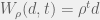
For some constant $p \geq 0$ (note that we can always assume the coefficient of $d$ is 1 (unless it is zero) by change of units and that there is no constant terms). However, the problem with above equation is that in the description of $U(v)$ the awesomeness parameter (for which we expect $d$ to be a proxy) and the time parameter do not interact linearly, but instead by multiples. Hence, it might be better to adopt a slightly more complicated $W$ that better reflect the structure of $U$ :

$W_\rho(d,t) = \rho^t d$

For some constant $0 \leq \rho \leq 1$ . This equation fits the form of $U(v)$ better and still satisfies the rationality constraints. Thus, in this part of the strategy space, the strategy of $S$ can be represented by a single parameter $\rho$ and the procedure would be to evaluate $W(v)$ for each vertex not in $F(S)$ and select uniformly at random from the ones that maximize it. Further, by making the strange assumption that $0^0$ is $1$ we can also use the equation to always select from the newest choices (note that this assumption is perfectly valid in the limit).

Deciding when to publish

The problem of deciding when to publish is much less clear cut than deciding what to read. We can make some rationality assumptions. For instance given sets $R_1, ..., R_t \subseteq F(S)$ with some $(v,n) \in R_i$ and $\Sigma(R_i) \geq U_{\mathrm{min}}$ for each $1 \leq i \leq t$ and knowing that the agent wants to publish one of these specific $t$ subsets this round (and no others), then by rationality agent $S$ should publish the subset $R_i$ that maximizes $\langle U \rangle_{R_i}$ where the new notation means that the average is taken over the elements of $R_i$ . However, this is a pretty weak constraint since the requirement of $(v,n)$ being present in all subsets is essential. Consider if there was instead two subsets $R$ and $R'$ both with $\Sigma(R), \Sigma(R') \geq U_{\mathrm{min}}$ and with $\langle R \rangle \geq \langle R' \rangle$ and no element in common between the two sets and the agent knew that he wants to publish one of these two sets. How does he decide which? Should he publish the better publication because it is better and it is best to get it out early? or should he publish the worser one now and wait for even better sources to add to the better publication? It is not clear if one is inherently better than the other in all cases, hence such a distinction would have to be part of the strategy space.

The only other rationality assumption that seems obvious to me is the one on reusable papers. Assume an agent has a subset $R$ that has no conflicts with other subsets (i.e. he is not deciding if he should publish other subsets over it) and he is simply deciding if he should publish $R$ now or wait one more turn and potentially sample another good paper. Now consider the condition $\alpha\beta\Sigma(R) \geq U_{\mathrm{min}}$ is met — then he should definitely publish now. Basically, the subset $R$ is so good, that he could republish it next turn even if he takes the $\beta$ hit of publishing it now. This condition is also pretty far-fetched.

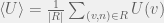
In general, I think the total strategy space for deciding when to publish is rather complicated. For this preliminary model we will have to drastically simplify it. One such simplification is to give each agent access to the mean utility of all the papers published so far — $\langle U^* \rangle$ and a parameter $q$ (for “quality”). Then, if the agent $S$ has a subset $R$ with $\Sigma(R) \geq U_{\mathrm{min}}$ and $\langle U \rangle_R \geq q \langle U^* \rangle$ then the agent publishes the subset. With this simplified model, we can then classify the total strategy space (reading and publishing) with two variables $\rho$ and $q$ . Simple… I hope.

Fitness: Impact or Awesomeness?

To study this question from an evolutionary game theory point of view, we need to define a fitness function. Here, there are two approaches, both involve looking at all the papers published by an author. One way is to look at impact: the number of citations to an author. The beauty of this approach is that we can use existing metrics based on citations such as mean citations, the h-index or some of the derivatives from it. On the other hand, since we have access to awesomeness, we could also use if for fitness (mean awesomeness of papers). The best thing is, we can combine all of the above, and by finding a good awesomeness metric we could compare how well impact factor ones (such as h-index) can recreate the ones based on awesomeness. That would tell us which impact factor system is best.

List of parameters

Let us look at all the parameters mentioned for the model with the `simplest’ assumptions:

$\alpha$ is the standard timescale and quantifies the decay rate of publications.
$\beta$ is a decay rate for reusing publications. A sort of milking factor. It should be related to $\alpha$ but not quiet a global time-scale since different agent strategies will have different frequency of publication and thus be affected by re-citations at a different rate compared to $\alpha$ . Thus, we can think of $\beta$ as a local time scale of agents. Although $\beta$ will be constant between agents, since each agent publishes at a different rate the interaction between the local timescale $\beta$ and the global $\alpha$ will be different for each type of agent.
$k$ is an amplification constant. It shows the factor by which the author amplifies the average awesomeness of the papers she read. We expect this factor to vary from field to field. However, to avoid a spiral into super useless papers, we will need $k \geq \alpha^{-m}$ where $m$ is the average time between publications for an average author.
$n_{\mathrm{new}}$ is the self-recycling boundary. Intuitively it accounts to the fact that when you write a paper you actually exhaust much more of the ideas corresponding to that paper, than you would from just seriously citing a paper. Hence, a meaningful range is $n_{\mathrm{new}} \geq 1$ .
$c$ is a constant that defines the threshold $U_{\mathrm{min}}$ in terms
of $\langle U^* \rangle$ . We need this constant to to be at least $c > 2$ to avoid the self-recycling problem. In particular, $c$ should give is a citations per paper scale. On average a researcher will have to sample $c$ or more papers from the graph before he can publish a new one.

These parameters along with the initial graph specify the environment in which agents live. Along with these, we have two parameters associated with agents:

$\rho$ is the agent’s reading habit. In particular, an agent with $\rho$ near $0$ places emphasis on fresh new results, and an agent with $\rho$ near $1$ concentrates on reading well established results.
$q$ is the agents quality standard. An agent with $q$ below $1$ wants to publish results as quickly as possible. An agent with $q$ above $1$ is willing to invest her time to create better results.

I expect $\alpha$ and $c$ to be two basic time scale parameters and basically set the citations-per-paper (average out-degree) and longevity of results. I would fix these in a reasonable range and instead fool around with $\beta$ , $k$ and $n_{\mathrm{new}}$ and see if different fields can be modeled with different values of these parameters. For the agents parameters, I expect the $q$ to produce a social dilemma type interaction between agents (in an evolutionary setting) and the $\rho$ to have a specific optimum value for each distribution over $q$ s. However, I would also not be surprised if these variables are somehow intertwined and self-regulating. In this model, if we set a min and max value for $q$ (say $0$ and $2$) then we will have four pure strategies:

NL — $\rho = 0, q = 0$ . A repeater of new results. Simply try to jump on new wagons with minor contributions.
NH — $\rho = 0, q = 2$ . An innovator: reads the newest literature and synthesizes it into a quality product.
OL — $\rho = 1, q = 0$ . A philosopher: concentrates on making quick minor contributions to already well studied fields.
OH — $\rho = 1, q =2$ . A theory builder: takes well established results and builds good things from them.

With that we can relabel he population strategy space as a vector on $S_3$ . It should be pretty suspicious that we have picked up an extra dimension in going from $\rho$ , $p$ to a tetrahedron. This is because $NL + OH$ is not linearly independent from $NH + OL$ . Hence, I expect that even though the simplest way of making an EGT model has $3$ dimensions, we still won’t see chaos. However, limit cycles do seem likely!

Is there any ways to simplify this model? Or is there essential parts missing that are needed to even be remotely useful? Do you know examples of similar models in the literature?

Filed under Models, Preliminary, Technical Tagged with citation network, networks and graphs