← Habitual selfish agents and rationality

Extra, Special Need for Social Connections →

Rationality for Bayesian agents

January 28, 2013 by Artem Kaznatcheev 9 Comments

One of the requirements of our objective versus subjective rationality model is to have learning agents that act rationally on their subjective representation of the world. The easiest parameter to consider learning is the probability of agents around you cooperating or defecting. In an one shot game without memory, your partner cannot condition their strategy on your current (or previous actions) directly. However, we don’t want to build knowledge of this into the agents, so we will allow them to learn the conditional probabilities $p$ of seeing a cooperation if they cooperate, and $q$ of seeing a cooperation if they defect. If the agents learning accurately reflects the world then we will have $p = q$ .

For now, let us consider learning $p$ , the other case will be analogous. In order to be rational, we will require the agent to use Bayesian inference. The hypotheses will be $H_x$ for $0 \leq x \leq 1$ — meaning that the partner has a probability $x$ of cooperation. The agent’s mind is then some probability distribution $f(x)$ over $H_x$ , with the expected value of $f$ being $p$ . Let us look at how the moments of $f(x)$ change with observations.

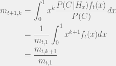
Suppose we have some initial distribution $f_0(x)$ , with moments $m_{0,k} = \mathbb{E}_{f}[x^k]$ . If we know the moments up to step $t$ then how will they behave at the next time step? Assume the partner cooperated:

$\begin{aligned} m_{t+1,k} & = \int_0^1 x^k \frac{ P(C|H_x) f_t(x) }{ P(C) } dx \\ & = \frac{1}{ m_{t,1} } \int_0^1 x^{k + 1} f_t(x) dx \\ & = \frac{ m_{t,k+1} }{ m_{t,1} } \end{aligned}$

If the partner defected:

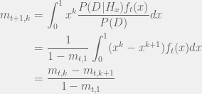
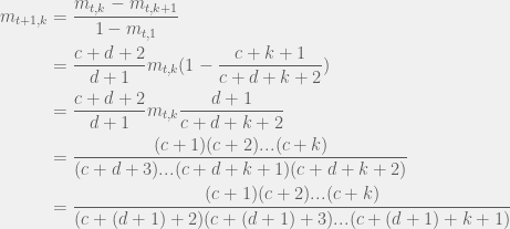
$\begin{aligned} m_{t+1,k} & = \int_0^1 x^k \frac{ P(D|H_x) f_t(x) }{ P(D) } dx \\ & = \frac{1}{ 1 - m_{t,1} } \int_0^1 (x^k - x^{k + 1}) f_t(x) dx \\ & = \frac{ m_{t,k} - m_{t,k+1} }{1 - m_{t,1} } \end{aligned}$

Although tracking moments is easier than updating the whole distribution and sufficient for recovering the quantity of interest ( $p$ — average probability of cooperation over $H_x$ ), it can be further simplified. If $f_0$ is the uniform distribution, then $m_{0,k} = \frac{1}{k + 1}$ . What are the moments doing at later times? They’re just counting, which we will prove by induction.

Our inductive hypothesis is that after $t$ observation, with $c$ of them being cooperation (and thus $d = t - c$ defection), we have:

$m_{t,k} = \frac{(c + 1)(c + 2)...(c + k)}{(c + d + 2)(c + d + 3)...(c + d + k + 1)}$ .

Note that this hypothesis implies that

$m_{t,k+1} = m_{t,k}\frac{c + k + 1}{c + d + k + 2}$ .

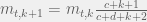If we look at the base case of $t = 0$ (and thus $c = d = 0$ ) then this simplifies to

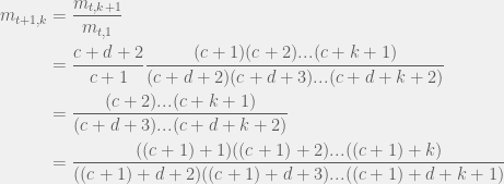
$m_{0,k} = \frac{1\cdot 2 \cdot ... \cdot k}{2 \cdot 3 \cdot ... \cdot k + 1} = \frac{k!}{((k + 1)!} = \frac{1}{k + 1}$ .

Our base case is met, so let us consider a step. Suppose that our $t + 1$ -st observation is a cooperation, then we have:

$\begin{aligned} m_{t + 1,k} & = \frac{ m_{t,k+1} }{ m_{t,1} } \\ & = \frac{ c + d + 2 }{c + 1} \frac{(c + 1)(c + 2)...(c + k + 1)}{(c + d + 2)(c + d + 3)...(c + d + k + 2)} \\ & = \frac{(c + 2)...(c + k + 1)}{(c + d + 3)...(c + d + k + 2)} \\ & = \frac{((c + 1) + 1)((c + 1) + 2)...((c + 1) + k)}{((c + 1) + d + 2)((c + 1) + d + 3)...((c + 1) + d + k + 1)} \end{aligned}$ .

Where the last line is exactly what we expect: observing a cooperation at step $t+1$ means we have seen a total of $c + 1$ cooperations.

If we observe a defection on step $t + 1$ , instead, then we have:

$\begin{aligned} m_{t + 1,k} & = \frac{m_{t,k} - m_{t,k+1} }{1 - m_{t,1} } \\ & = \frac{ c + d + 2 }{d + 1} m_{t,k}( 1 - \frac{c + k + 1}{c + d + k + 2}) \\ & = \frac{ c + d + 2 }{d + 1} m_{t,k} \frac{d + 1}{c + d + k + 2} \\ & = \frac{(c + 1)(c + 2)...(c + k)}{(c + d + 3)...(c + d + k + 1)(c + d + k + 2)} \\ & = \frac{(c + 1)(c + 2)...(c + k)}{(c + (d + 1) + 2)(c + (d + 1) + 3)...(c + (d + 1) + k + 1)} \end{aligned}$

Which is also exactly what we expect: observing a defection at step $t+1$ means we have seen a total of $d + 1$ defections. This completes our proof by induction, and means that our agents need to only store the number of cooperations and defections they have experienced.

I suspect the above theorem is taught in any first statistics course, unfortunately I’ve never had a stats class so I had to recreate the theorem here. If you know the name of this result then please leave it in the comments. For those that haven’t seen this before, I think it is nice to see explicitly how rationally estimating probabilities based on past data reduces to counting that data.

Our agents are then described by two numbers giving their genotype, and four for their mind. For the genotype, there is the values of $U$ and $V$ that mean that the agent thinks it is playing the following cooperate-defect game:

$\begin{pmatrix} 1 & U \\ V & 0 \end{pmatrix}$

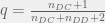For the agents’ mind, we have $n_{CC}, n_{CD}$ which is the number of cooperations and defections the agents saw after cooperation, and $n_{DC}, n_{DD}$ is the same following a defection. From these values and the theorem we just proved, the agent knows that $p = \frac{n_{CC} + 1}{n_{CC} + n_{CD} + 2}$ and $q = \frac{n_{DC} + 1}{n_{DC} + n_{DD} + 2}$ . With these values, the agent can calculate the expected subjective utility of cooperating and defecting:

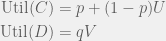
$\begin{aligned} \text{Util}(C) & = p + (1 - p)U \\ \text{Util}(D) & = qV \end{aligned}$

If $\text{Util}(C) > \text{Util}(D)$ then the agent will cooperate, otherwise — defect. This has a risk of locking an agent into one action forever, say cooperate, and then never having a chance to sample results for defection and thus never update $q$ . To avoid this, we use the trembling-hand mechanism (or $\epsilon$ -greedy reinforcement learning): with small probability $\epsilon$ the agent performs the opposite action of what it intended.

The above agent is rational with respect to its subjective state $U,V,p,q$ but could be acting irrationally with respect to the objective game $\begin{pmatrix}1 & X \\ Y & 0 \end{pmatrix}$ and proportion of cooperation $r$ .

Filed under Analytic, Models, Preliminary, Simulation, Technical Tagged with bayesian, learning, rationality

About Artem Kaznatcheev
From the Department of Computer Science at Oxford University and Department of Translational Hematology & Oncology Research at Cleveland Clinic, I marvel at the world through algorithmic lenses. My mind is drawn to evolutionary dynamics, theoretical computer science, mathematical oncology, computational learning theory, and philosophy of science. Previously I was at the Department of Integrated Mathematical Oncology at Moffitt Cancer Center, and the School of Computer Science and Department of Psychology at McGill University. In a past life, I worried about quantum queries at the Institute for Quantum Computing and Department of Combinatorics & Optimization at University of Waterloo and as a visitor to the Centre for Quantum Technologies at National University of Singapore. Meander with me on Google+ and Twitter.

9 Responses to Rationality for Bayesian agents

Pingback: Quasi-magical thinking and superrationality for Bayesian agents | Theory, Evolution, and Games Group
Pingback: Evolving useful delusions to promote cooperation | Theory, Evolution, and Games Group
Pingback: Cooperation through useful delusions: quasi-magical thinking and subjective utility | Theory, Evolution, and Games Group
Pingback: Cataloging a year of blogging: from behavior to society and mind | Theory, Evolution, and Games Group
Pingback: Useful delusions, interface theory of perception, and religion. | Theory, Evolution, and Games Group
John says:

January 8, 2015 at 15:04

I really want to understand the details of this article so that I can further understand the subjective/ objective reality model. I hope that you can help.

1. For the first paragraph, I do not understand the setup. In the beginning what is going on? what exactly is being modeled? And why this statement, ” If the agents learning accurately reflects the world then we will have p = q.” ?

2. Is H a random variable and f the mass function? If so what is the sample space or the experiment? i.e. P(H=x) = \int_0^1 f(x)dx ??
I do not understand, ” The agent’s mind is then some probability distribution f(x) over H_x, with the expected value of f being p.”

3. Starting with the third paragraph, f_0 is the initial distribution of what? In the formula for m_{0,k} should that be f or f_0? Where do the moments come from?

thanks john

Reply
- Artem Kaznatcheev says:
  
  January 8, 2015 at 17:06
  
  Thank you for your interest. The details of this article are not necessary for the subjective/objective rationality model since the main results hold with or without the mechanism discussed here in place (and would also hold for reasonable variations of this mechanism). However, I’ll answer your questions for completeness.
  
  [1] The model is the following, a focal agent (call her Alice) interacts with some other agent (call him Bob). Alice and Bob decide and announce simultaneously if they will cooperate or defect. In order to make her decision, Alice wants to have some idea of the probability that Bob will decide to cooperate; she bases this on Bayesian learning from previous interactions with other agents.
  
  Thus, she wants to estimate two probabilities: p is the probability that Bob will cooperate if Alice cooperates and q is the probability that Bob will cooperate if Alice defects. Note that since Alice and Bob make their decision simultaneously, Alice’s choice cannot actually affect Bob’s choice; so with proper reasoning and perfect knowledge, one would know that p = q. However, we allow for the possibility of agents not coming to this conclusion, so that we have a framework in which we can model things like quasi-magical thinking.
  
  [2] That is correct. The state space of hypotheses $\{H_x | 0 \leq x \leq 1\}$ , the state space of data is if an agent cooperated or defected. The agents is a Bayesian reasoner that has some beliefs about each hypothesis $H_x$ being true, thus their ‘mind’ is simply all that information together; in other words their minds is the probability distribution f over $H_x$ . From this probability distribution over hypotheses, they need to know the expected probability that Bob will cooperate; that is simply the mean of f.
  
  [3] The prior distribution that the agent has before any experience. In the first calculation, it is treated generally (so it can be any distribution you want) and then after paragraph 4, I consider the special case of $f_0$ being the uniform distribution. The moments come from the probability distribution.
  
  I hope this was helpful. You should take a look at our paper, where this is also discussed.
  
  Reply
  - jcleve72 says:
    
    January 26, 2015 at 19:20
    
    Thanks for your response.
    
    [2] Let W ={ (x_i)| x_i = C or D}. Each (x_i) is a finite (infinite) sequence that represents an iterated game played between A and B OR W could be a collection of many such games played by many players. In any event H: W —> [0,1] by H(w) = longterm proportion of C’s or the probability of obtaining a C given that A or first player played a C.
    
    Then H is a random variable and P( a <= H <= b) = int_a^b f(x)dx.
    
    Is this the setup?
    
    [3] Also m_{0,k} = E_{f_{0}}[x^k]?? In other words what is the relationship between f and f_0? Also could you go thru a few of the steps in your determination of m{t+1,k}. In particular, how to get the m_{t,1} in the denominator.
    
    Thanks John
    
    Reply
Pingback: Rationality, the Bayesian mind and its limits | Theory, Evolution, and Games Group